Replacing values in a string

I received a request for help in a comment on one of my blog posts.

I don’t normally offer a helpdesk service, but I found the problem both interesting and challenging, so I thought I’d give it a go.

The question was:

“Hope you could help me here. I want to sort out free format text object which contains keywords. For example,

aaa/bbb/blue
ccc/ddd/yellow
eee/fff/red
ggg/hhh/xyz

Find “blue” from the object and replace the entire object with “azul”, find “yellow” then replace with “amarillo”, “red” into “rojo”. When neither “blue”, ”yellow” nor ”red” was found, replace the object with “not found”. So in the above example, “ggg/hhh/xyz” will be displayed as “not found”.

Thanks in advance for your assistance.”

Not being familiar with the entire data set or possible range of values, I need to make a few assumptions.

I assume you want to see the following output:

aaa/bbb/azul
ccc/ddd/amarillo
eee/fff/rojo
ggg/hhh/not found

I also assume that the position of the second forward slash may change.

If my assumptions are correct, we can move forward. If not, let me know!

When faced with such a problem, I like to break it down into logical steps, building up the formula until I get the result I’m after.

Now I’m assuming that you

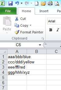
For those that want to follow, I created a sample data file in Excel:

I then created a report using the Excel file.

The challenge is to replace the text after the second forward slash with another value depending on its content.

So lets start.

Using the Pos() function, you can determine the position of the first forward slash:

This gives us 4.

We need to find the position of the second slash, so we create a new string using the output from the function Pos(<F1>,”/”). To do this we use substr().

Substr allows us to take a part of string. To use this we pass in the data value, its start position and the length of the string to return.

For our example, we will use the following formula:

SubStr(<F1> ,Pos(<F1> ,”/”)+1 ,10)

If you are using Web Intelligence, the following formula will work:

SubStr([F1];Pos([F1];”/”)+1;10)

With this formula we are saying:

Return a substring of <F1>, stating in position 5, and bring back 10 characters.

Notice I said position 5 (we added +1). The reason for this is that we want to bring back the string after the first forward slash.

We end up with the following results:

Now we have a new string to work with, we need to find out the position of the forward slash in this string. We use:

Pos(SubStr(<F1> ,Pos(<F1> ,”/”)+1 ,10) ,”/”)

If you are using Web Intelligence, the following formula will work:

Pos(Substr([F1];Pos([F1] ;”/”)+1;10);”/”)

If we put these two formulas together, our result should be everything after the second forward slash:

If you are using Web Intelligence, the following formula will work:

Substr(Substr([F1] ;Pos([F1] ;”/”)+1 ;10) ;Pos(Substr([F1] ;Pos([F1] ;”/”)+1 ;10) ;”/”)+1 ;10)

We now have a formula to determine the character string after the second forward slash.
We can now start work on the real solution. We want to check for three possible values. If none of these values are found, we return a fourth ‘catch all’ value.

To perform this check, we use an If() function together with the Else command.

We also make use of the Replace() function within the statement to swap out the relevant values.

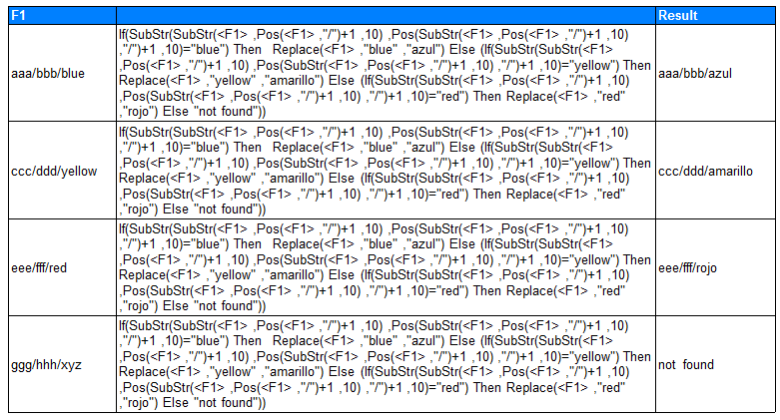
So we end up with the following formula:

If(SubStr(SubStr(<F1> ,Pos(<F1>,”/”)+1 ,10) ,Pos(SubStr(<F1> ,Pos(<F1> ,”/”)+1 ,10) ,”/”)+1 ,10)=”blue”) Then Replace(<F1> ,”blue” ,”azul”) Else
(If(SubStr(SubStr(<F1>,Pos( <F1>,”/”)+1 ,10) ,Pos(SubStr(<F1> ,Pos( <F1>,”/”)+1 ,10) ,”/”)+1 ,10)=”yellow”) Then Replace(<F1> ,”yellow” ,”amarillo”) Else
(If(SubStr(SubStr(<F1> ,Pos( <F1>,”/”)+1 ,10) ,Pos(SubStr(<F1> ,Pos( <F1>,”/”)+1 ,10) ,”/”)+1 ,10)=”red”) Then Replace(<F1> ,”red” ,”rojo”) Else
“not found”))

If you are using Web Intelligence, the following formula will work:

If(Substr(Substr([F1] ;Pos([F1] ;”/”)+1 ;10) ;Pos(Substr([F1] ;Pos([F1] ;”/”)+1 ;10) ;”/”)+1 ;10)=”blue”; Replace([F1] ;”blue” ;”azul”); (If(Substr(Substr([F1] ;Pos([F1] ;”/”)+1 ;10) ;Pos(Substr([F1] ;Pos([F1] ;”/”)+1 ;10) ;”/”)+1 ;10)=”yellow”; Replace([F1] ;”yellow” ;”amarillo”); (If(Substr(Substr([F1] ;Pos([F1] ;”/”)+1 ;10) ;Pos(Substr([F1] ;Pos([F1] ;”/”)+1 ;10) ;”/”)+1 ;10)=”red”; Replace([F1] ;”red” ;”rojo”); “not found”)))))

Note: If you don’t want to see the whole string and simply want “azul”, “amarillo”, “rojo” or “not found” displayed, then change the Replace command slightly as follows:

Replace(<F1> ,<F1> ,”azul”) 

or in Web Intelligence:

Replace([F1];[F1];”azul”) 

So we have ended up with quite a long formula composed of several functions:

If()
Substr()
Pos()
Replace()

Remember:

We couldn’t just do a Replace(), as there are multiple values to replace.

We couldn’t use an If() and a Replace() function, as the data set and length is not known in advance. The position of the second forward slash may change.

Therefore we used the Pos() function to find the position of the second slash, and use the If, Substr and Replace functions to replace the contents following that second slash.

I hope you found this post helpful. If you have any comments, do let me know.

How to handle DIV/0 errors in Web Intelligence

A short and simple post about handling DIV/0 errors.

To handle DIV/0 errors, use the If() and IsError() functions.

IsError() will return a true or false value depending on the item being evaluated. Wrap this with an If() statement and you can evaluate the formula as normal is if it is ok, or return a message to the user if there is an error:

=If(IsError(15/0);”Error in formula”;15/0)

How to insert th into a date field

Is it possible to enter th/nd/rd/st into the date field on a report?

This was the question recently asked of me by a client.

Unfortunately there isn’t a specific date format you can use to give you this information. However, with the use of a number of functions, you can build up a formula to achieve the desired result.

Lets break this down into small steps:

Step 1:

Let say we start with a date field with the following value: 09/Jul/2013 (dd/Mmm/yyyy).

The day part of this field will determine the text to append the day part of the date. There are four potential apend options depending on the day selected:

Day Number – Text To Append
1 – st
2 – nd
3 – rd
4 – th
5 – th
6 – th
7 – th
8 – th
9 – th
10 – th
11 – th
12 – th
13 – th
14 – th
15 – th
16 – th
17 – th
18 – th
19 – th
20 – th
21 – st
22 – nd
23 – rd
24 -th
25 – th
26 – th
27 – th
28 – th
29 – th
30 – th
31 – st

 As we want to query the day portion of the date, we need to use the Substr() function. This is used to bring back the first two characters of the date from a start position of one. But note: As our input value is a date field, we need to convert the date to a string. We do this using the FormatDate() function.

We end up with the following formula:

=Substr(FormatDate(CurrentDate();”dd/mm/yyyy”);1;2)

which returns 09

Step 2:

Now that we have the day portion, we want to identify which value to append. There are four possible values. Days 1 and 31 will have ‘st’ appended. Day 2 will have ‘nd’ appended. Day 3 will have ‘rd’ appended. And every other value will have ‘st’ appended.

We can create this formula by building on the previous statement and using the If() function. In our example we have to use a nested If() statement to evaluate three conditions. If the test doesn’t match any of the three conditions, it will default to a fourth option:

=If (Substr(FormatDate(CurrentDate();”dd/mm/yyyy”);1;2) InList (“1″;”01″;”21″;”31″);”st”;If (Substr(FormatDate(CurrentDate();”dd/mm/yyyy”);1;2) InList (“2″;”02″;”22″);”nd”;
If (Substr(FormatDate(CurrentDate();”dd/mm/yyyy”);1;2) InList (“3″;”03″;”23″);”rd”;”th”)))

You will notice that as well as checking for any days prefixed with a zero, I am also checking for the same value without a preceeding zero.

Running the above formula for 09/Jul/2013 will return the result: th as it is the 9th today.

Step 3:

We then break out the other components of the date field to extract the month and year parts. We will use these formulas shortly:

=Substr(FormatDate(CurrentDate();”dd/Mmm/yyyy”);4;3)

This returns Jul.

Step 4:

=Substr(FormatDate(CurrentDate();”dd/mm/yyyy”);7;4)

This returns 2013.

We now have all the components we need to generate a date string which incorporates the th/nd/rd/st text.

Step 5:

Here we put it all together using several Concatenation() statements:

=Concatenation(Concatenation(Concatenation(Concatenation(Concatenation(Substr(FormatDate(CurrentDate();”dd/mm/yyyy”);1;2);
If (Substr(FormatDate(CurrentDate();”dd/mm/yyyy”);1;2) InList (“1″;”01″;”21″;”31″);”st”;
If (Substr(FormatDate(CurrentDate();”dd/mm/yyyy”);1;2) InList (“2″;”02″;”22″);”nd”;
If (Substr(FormatDate(CurrentDate();”dd/mm/yyyy”);1;2) InList (“3″;”03″;”23″);”rd”;”th”))));
” “);Substr(FormatDate(CurrentDate();”dd/Mmm/yyyy”);4;3));” “);
Substr(FormatDate(CurrentDate();”dd/mm/yyyy”);7;4))

You will notice that I have included spaces in between the individual date components. Without this all the data will be bunched up and won’t read nicely.

We end up with the following result:

09th Jul 2013

Bonus:

The icing on the cake is the removal of the leading zero from the day part of the date. We can acheive this by performing a check on the date field using an If() statement. If the day part of teh field starts with a zero, we start our substr() statement at position 2 and return 1 character. Otherwise we start in position 1 and return 2 characters:

=Concatenation(Concatenation(Concatenation(Concatenation(Concatenation(If(Substr(FormatDate(CurrentDate();”dd/mm/yyyy”);1;1)=”0″;Substr(FormatDate(CurrentDate();”dd/mm/yyyy”);2;1);Substr(FormatDate(CurrentDate();”dd/mm/yyyy”);1;2));
If (Substr(FormatDate(CurrentDate();”dd/mm/yyyy”);1;2) InList (“1″;”01″;”21″;”31″);”st”;
If (Substr(FormatDate(CurrentDate();”dd/mm/yyyy”);1;2) InList (“2″;”02″;”22″);”nd”;
If (Substr(FormatDate(CurrentDate();”dd/mm/yyyy”);1;2) InList (“3″;”03″;”23″);”rd”;”th”))));
” “);Substr(FormatDate(CurrentDate();”dd/Mmm/yyyy”);4;3));” “);
Substr(FormatDate(CurrentDate();”dd/mm/yyyy”);7;4))

This gives us the following result:

9th July 2013

Bear in mind that adding the th/nd/rd/st text means this field is now a string an not a date. The effect of this is that you won’t be able to use any Date specific functions on this new field. You can overcome this by performing any date calculations prior to appending the text.

So while not the most elegant of solutions, it is perfectly possible to achieve. Does anyone know a more elegant solution?

How to remove a specified number of characters from a string

A question was recently posted on the excellent Business Objects forum about how to remove a variable number of characters from the front of a string up to a specified character.

In this example the data was CKI=ICD9!250.02 and the user required all the values after the ! returned, i.e. 250.02. They also went on to state that the number of characters after the 250.02 may vary in length.

Interesting. What immediately sprang to mind was the MID() function available in Excel. However, this is not available in Web Intelligence.

However, Web Intelligence does provide us with the Right(), Length() and Pos() functions. Used together in a formula, we can get the desired result.

The first step is to determine the length of the character string. We are told it could be a variable length, so lets determine its length:

=Length([Object])

In this case we get 15.

Next we determine the position of the exclamation mark using Pos():

=Pos([Object];”!”)

This gives us 9

Finally, we use the Right() function. This takes two values; an input string and the number of characters to retrieve from the right of the string.

The second part is built up using the Length and the Pos calculations we made earlier.

=(Length([Object])-Pos([Object];”!”))

This gives us a value of 6. We should therefore count six characters from the left of the character string.

Putting this all together we create this formula:

=Right([Object];(Length([Object])-Pos([Object];”!”)))

…giving us the desired result of 250.02

Alternate row shading in Webi/Deski

One of our Business Objects Blog readers recently asked a question about alternate row coloring in Web Intelligence.

“Hi. I have a question on alternating row colors in Webi. I went to the properties and set 2 for the frequency in the “Alternate Row/Column colors” and have the specified color. Do you know why it’s showing as one color and not alternating the colors with white in between? Is there any other settings I need to change.
I’d appreciate your opinions. Thanks, Sam.”

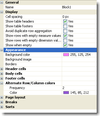
I’m not sure about everyone else, but I have found that selecting a colour from the drop down list doesn’t appear to work for me. Instead I determine the RGB codes and entered them in the Color row. The Frequency of the alternate row is set to 2. This produces the desired alternate row effect.

Before this feature was available, I implemented alternate row shading via the use of a variable and the alerter feature. I’ll describe it here, both for Web Intelligence and Desktop Intelligence.

Web Intelligence alternate row shading

Through the use of the Odd() and LineNumber() functions, we can create a statement that can be used by an alerter to create our alternate row shading.

The steps to create this are as follows:

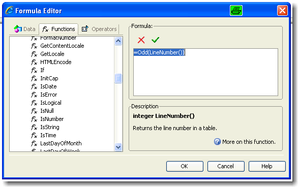
In the Formula Editor, create a new statement as follows:

=Odd(LineNumber())

(You may need to temporarily add a new column to your table to do this. We can delete this later.)

The Odd function requires that you pass in a numeric value. It will determine if that value is odd. If it is, it will return a 1. If it is not, it will return a 0.

The LineNumber function simply returns the line number for each row in a table.

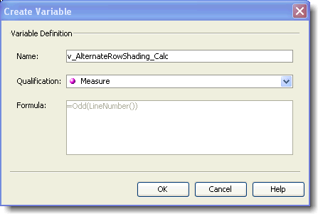
Put the statement into a variable, e.g. v_AlternateRowShading_Calc using the Create Variable icon.

Highlight the column/s you wish to apply alternate row shading and click the Alerter icon.

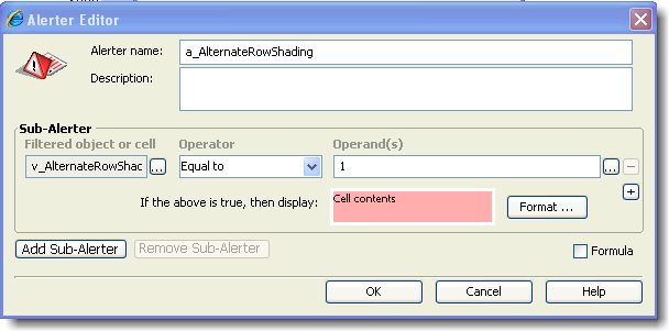
Create a new alerter and give it a meaningful name, e.g. a_AlternateRowShading.

In the cell ‘Filtered object or cell’, use the button to find your newly created variable. Chose ‘Select an object or variable’ from the drop down list.

Click OK.

Ensure the operator is set to ‘Equal to’

In the Operand(s) cell, type 1.

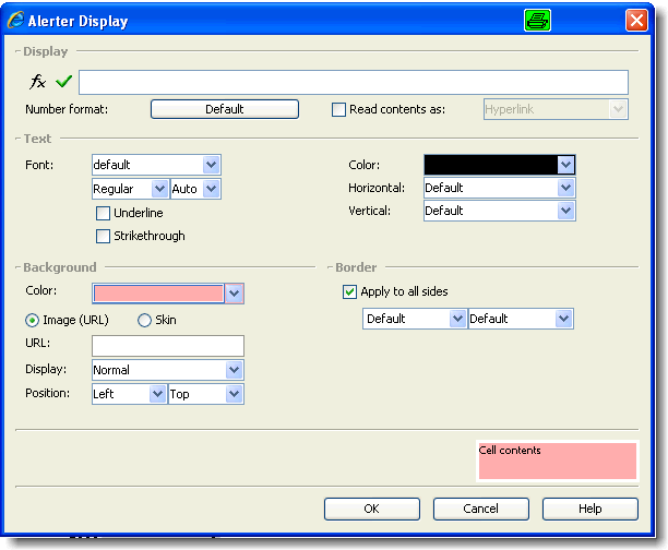
Then click the ‘Format’ button to set the format of the cell. In this case I’ve changed the background color to pink and the font color to black.

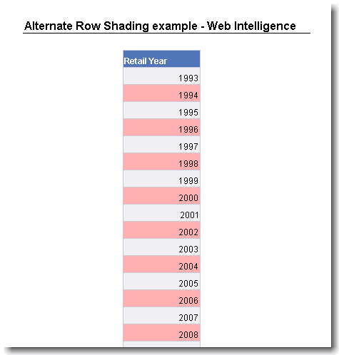
Click OK, and OK again. The table should now have alternate row shading.

You can now safely remove the column containing the v_AlternateRowShading variable.

Desktop Intelligence alternate row shading

A similar process to the Web Intelligence method.

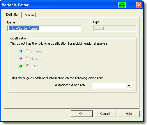
Create a new variable using the Variable Editor.

In the Definition tab, give it a meaningful name such as v_LineNumberFormat.

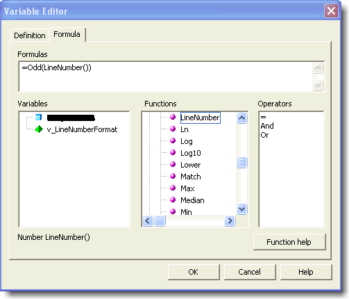
In the Formula tab, enter =Odd(LineNumber())

Highlight the column/s you wish to apply alternate row shading and click the Alerter icon.

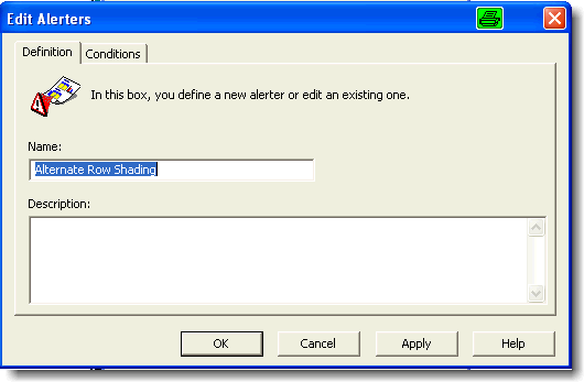
Create a new alerter and in the Definition tab, give it a meaningful name, e.g. a_AlternateRowShading.

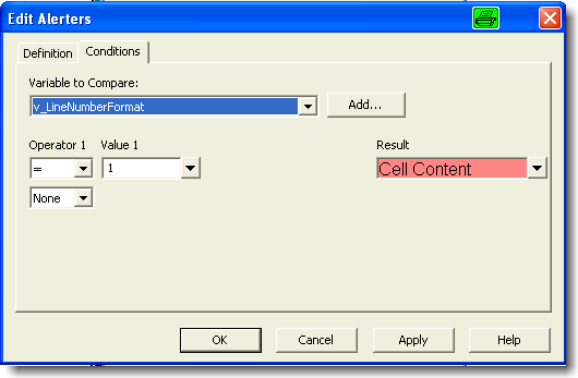
In the Conditions tab, select v_LineNumberFormat from the drop down list of variables to compare.

In the cell ‘Filtered object or cell’, use the button to find your newly created variable. Chose ‘Select an object or variable’ from the drop down list.

Ensure Operator1 is set to ‘=’

In the Value 1 cell, type 1.

Then click the ‘Result’ drop down button, and select Format. Set the format of the cell. In this case I’ve changed the background color to pink and the font color to black.

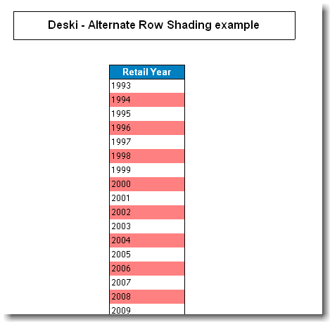
Click OK, Apply and OK again. The table should now have alternate row shading.

Sam – I hope this helps to answer your question. Thanks for submitting a question to the BOBJBLOG!

Practical Business Objects Developer Tips

I’ve been meaning to write up a good practice guide for Business Objects developers for some time now.

I have finally managed to find some time to put together a list of tips I’ve used over the years. I hope you find the following list of tips useful in some small way.

If, after reading this article, you come away with something new, then I’ll be very happy.

I’m going to keep this post going for a while, adding to it as and when I can. But more importantly, I’d love for you to share your developer tips. I know there is a wide community of Business Objects experts out there, so please help develop this list so we can all benefit from our shared experiences.

If you’d like to share a tip or two, please add a comment to the post. I’ll then add it to the main list and give you a name check!

Universe Designer Application

• Use business terminology for all universe objects – always. The universe is the semantic layer between the business and IT.
• Wherever possible, and certainly for measures and calculated objects, add a description to the object.
• Ensure your object is formatted correctly. Pay particular attention to dates and numeric fields.
• Create filtered prompts wherever possible. Anything which can help the user get their data more efficiently helps. Remember to allow the selection of all data.
• Ensure your List of Values (LOV) is sorted. Don’t assume it will be.
• Don’t create a LOV on a measure.
• If you have to create a LOV on a dimension with many data items, consider grouping those items.
• Group your universe objects into a logical order. Create something that the business will understand and be familiar with.
• Create different time periods – users like to compare current year to date to last year to date, quarter to date, month to date, etc.
• Contexts – these can be incredibly useful. But they can become terribly confusing to the end user. If you really have to put in a context, do so, but make sure it has a meaningful name and description. If your user is presented with a context prompt box, it should be absolutely clear to them which context to choose. If it isn’t, you need to revisit your context or approach. The purpose of the tool is to help the end user get their results. Remember that.
• For fields based on free form input text, consider trimming the field. Profiling your data beforehand should help you identify these fields.

Reporter Application

The Query Panel

• Only use objects that you are going to use in your report.
• Put the objects in the order that you would like them sorted on the report if possible.
• Move your measures to the end.
• Use pre-defined (universe) filters if available.
• Avoid hard coding values wherever possible – use prompts instead.
• If you are not familiar with your data set, restrict the number of rows returned by your original query. If you are happy with the result set, you can remove this restriction. The last thing you need is to run the mother of all queries.
• Make prompts meaningful. If you are prompting for a date, include an example of the expected format. If a user can enter a ‘*’ to select all values, say so.
• Get the server to do the work rather than the report. Not all end user PC’s are high spec.
• If you are going to use multiple queries, give each query a meaningful name.

Report Design

• Create a report header tab/page – this should list the report title, parameters used, descriptions, values entered at the prompts, last refreshed date.
• Ensure the report opens on this header page. This should result in a faster opening report.
• Keep the report look and feel the same throughout – table positions, headers, fonts and colours.
• For tables that span across several pages, repeat the header on every new page.
• Dates – who is your target audience? US and UK data formats differ. If you do not know who your audience is, or if it is a worldwide audience, specify the format of the dates in the header page of the report or the column heading.
• Decimal places – how many decimal places do you need to report on? How many decimal places are used in the calculation?
• When working with large numbers with several digits, consider dividing by a thousand or a million. Ensure the report states that you are reporting in that way.
• Include error handling in any calculations performed on the fly. Pay special attention to DIV/0 errors. Use the IsError function. This post may help.
• For all new formulas you create, consider putting them into a variable to allow reuse and easy maintenance. Prefix the variable name with v_ to make them easily identifiable.
• Include a cell at the bottom of your report to show the last refreshed date.
• Build in a very visible partial refreshed alert. All too often that yellow triangle is overlooked by users. This post may help.
• Number your report pages. ‘Page n of n’ works well.
• Give the report a meaningful name. Include a description. Keywords are helpful too for searching.
• Consider a numbering scheme for your reports. E.g. first digit represents dept/function, second digit represents area, etc. E.g. 104 – Sales Report London, 105 Sales Report New York, 204 – Finance Report London. This will allow rapid identification of a report series.
• Use autofit width or wrap text for longer fields. If you only want to display the first n characters of a field in a report, create a formula to do so (e.g. Left(,20))
• Be consistent with your fonts.
• Use a sensible font like Arial. Some of the more fancy fonts do not print too well, especially if a smaller size font is used.
• Consider how your users will use the report. If they tend to print reports, and they do not have a colour printer, avoid colour on your report. Colours on report don’t lend themselves well to output on a black and white printer. If you must use shading, consider greyscale. If you users only view reports on screen, colours can help identify sections of data.
• Use alerters. These are a great tool for bringing data to the users attention. Given them a meaningful name and description.
• Optimise your report for speed – reduce or eliminate unused formulas, alerters and formatting. Keep it simple.
• Consider the use of section breaks to break up large tables. These can be easily searched in the side panel.
• Before publishing or releasing a report to production, do a print preview. Does the report print out as you’d expect? Do you need to save the report in landscape. Also save to Excel. Are any fields appearing incorrectly formatted?
• Big reports – Do your users really need that 100 page report? Really? If all they are after is a data dump, a more efficient way to deliver this is to write a piece of SQL code and save the result as a CSV file. But always ask why they want a data dump in the first place. What they do with the data? BOBJ is a powerful tool. Show them how to do what they want to do. Use it.
• Save your work regularly. You never know when the power will go, or an application will crash. If you have spent the last couple of hours working on a report, it’s not going to hurt to hit that save button. I normally save every significant change as a new version. Once I have a report ready for production, I’ll delete those versions.
• Images such as a corporate logo can be inserted into reports. But keep the images small. Use a file format that compresses the image to a sensible size. Don’t even think about inserted a large 1mb image on every page. This post may help.
• Make use of multiple tabs in the report. However, avoid hard coding date values in these tabs. You will have to maintain these later.
• If you have a particularly complex report, add a tab that provides the detail behind the report. This will aid future developers.
• If you have one set of users that simply love to play with data, and others who want a formatted report, consider adding a Data Dump tab at the end of your report. This should be a simple table with zero formatting.
• Prior to release to UAT/Production, delete any unused variables and formulas.
• If running multiple queries, ensure the relevant dimensions are linked.
• Purge your report before release to production. The data may be obsolete by the time the user retrieves the report and it will be bigger than it needs to be.
• For corporate reports, consider developing a standard report template
• If your company reports in several currencies, ensure the measures on your report are clear as to what currency is being used.
• Avoid falling into the trap of creating several versions of essentially the same report. Remove hard coding and make the report as generic as possible. Use prompts. If a user wants a new field, can it be added to an existing report or do you need to create a duplicate with the new field?
• If you use graphs, keep them simple. Avoid 3D graphs. Read a good book on Data Visualisation to understand how to deliver data in a visual format. This post may help.
• If you have multiple tabs in a section, ensure that they are positioned relative to each other. Same applies to floating cells. Ensure they are relative to something so that they don’t overlap with other objects on your report.
• Percentages should be calculated within the report to ensure it is in context.
• If you create a grouped variable, you need to check that all possible values for that dimension are grouped. If not, the next time you run that report, you may find data that is not sitting in a group. This could lead to misleading results.

Handling formula errors in Web Intelligence

Don’t you just hate it when you see a report with DIV/0 errors?

Thankfully, Web Intelligence provides us with a function to handle these types of errors, allowing us to provide a more meaningful message.

Lets look at IsError

IsError() is a function which will return a boolean value.

A 1 is returned is the formula being evaluated is in error. A 0 if there is no error.

This function is particularly useful when embedded into an IF statement:

Lets assume x = 6 and y = 0

IF (IsError(x/y);”The y object is zero – a DIV/0 error has occured”;(x/y))

In this example, the statement x/y is being evaluated within the IsError function:

6/0

As you can’t divide by zero, a DIV/0 error has occured and a 1 is returned by the IsError statement.

The IF statement then presents one of two outcomes depending on this boolean value.

In the case of an error, the user is presented with some meaningful text:

“The y object is zero – a DIV/0 error has occured”

If we change the y value to 3, the IsError function returns 0 – no error, and the second part of the IF statement is evaluated: x/y – which gives us a value of 2.

It is good practice to include error handling into your reports, particularly when you are performing any type of division task. Wrapping an If IsError check around your formula ensures that these type of errors are handled in the correct manner and should help the user identify how the problem can be fixed.

How to calculate the number of days in a month in WebIntelligence

A quick method of determining the number of days in a month in WebIntelligence is through the use of the LastDayOfMonth function.

For a specified date, the LastDayOfMonth will give you the last day in that month.

=LastDayOfMonth(CurrentDate())

To extract the number of days, we want to use the first two digits of this result. The following formula will acheive that:

=Left(FormatDate(LastDayOfMonth(CurrentDate());”dd/MM/yyyy”);2)

We’ve added two functions here. The first is FormatDate. LastDayOfMonth returns a value held as a date field. We ultimately want the first two digits of this field. However, using the Left() function means we have to have a string input, not a date input. We have to convert the input into a string format first.

This requires two steps.

The first is to convert the LastDayOfMonth value into a string. We do this using the FormatDate function:

=FormatDate(LastDayOfMonth(CurrentDate());”dd/MM/yyyy”)

We now have a string.

We then extract the first two digits to give us the number of days in a month:

=Left(FormatDate(LastDayOfMonth(CurrentDate());”dd/MM/yyyy”);2)

If we want to subsequently use this in a calculation, we need to further manipulate this value and convert it to a number. This is achieved using the ToNumber function:

number ToNumber(string number_string)

This takes a string value and converts it to a number.

In our case, we create the following formula:

=ToNumber(Left(FormatDate(LastDayOfMonth(CurrentDate());”dd/MM/yyyy”);2))

We now have the number of days for a particular month that we can use in our calculations.

Missing FirstDayOfMonth() function…

Sadly, there isn’t a function to determine the first day of the month. However, we have a method of extracting the last day of the month using LastDayOfMonth() and using the formulas described above, we can work out the first day:

=RelativeDate(LastDayOfMonth(CurrentDate());-ToNumber(Left(FormatDate(LastDayOfMonth(CurrentDate()) ;”dd/MM/yyyy”);2))+1)

Despite looking complex, we are subtracting the number of days in the month (plus one) from the last day of the month. If we subtracted the total number of days in the month, we would end up with the last day of the previous month! We don’t want this. So we add a 1 to give us the first day.

Also note that in order to subtract days, we have prefixed the ToNumber function with a minus symbol.

Update:

Hat tip to JB for pointing out that we can avoid the string conversion by using the DayNumberOfMonth function. 

Hence, to calculate the last day of the month:

=DayNumberOfMonth(LastDayOfMonth(CurrentDate()))

And the first day of the month:

=DayNumberOfMonth(RelativeDate(CurrentDate(); 1-DayNumberOfMonth(CurrentDate())))

How to convert a string prompt into a date in WebIntelligence

 There are occasions where we need to prompt the user for a date. This can be done using the prompt functionality in the query panel.

We can display the value entered by the user at the prompt using the UserResponse function.

The UserResponse function is made up of two parts:

string UserResponse(string data_provider;string prompt)

The first part is the Data Provider that contains the prompt that you want to use. This is an optional field and is only required if your report contains multiple data providers. If you are only using one data provider, ignore this first part.

The second part is the EXACT text of your prompt string.

This needs to be a perfect match to your prompt. A way to ensure this is to copy and past the prompt string before you refresh the report.

When refreshed, the function will return the prompt value.

Note that the value returned from the UserResponse function is a string. Despite the value being shown as a date, the value is stored as a string. This means we are not able to perform date calculations on this field as it stands. The error message that will be shown is:

 

To overcome this, we expand the formula slightly and nest the UserResponse function inside a ToDate function.

The ToDate function is made up of two parts:

date ToDate(string input_string;string date_format)

The first part is the input string (in our case the UserResponse formula), and the second part is the format of the input. Note that the format has to match the input exactly.

We end up with the following formula:

 =ToDate(UserResponse(“Enter Date:”);”dd/mm/yyyy”)

At this stage, the user prompted date is converted to a date format and can be used in date calculations.

Bonus:

If you subsequently want to display the user prompted date in a specific date format, we would nest the formula further and include a FormatDate function:

string FormatDate(date date_to_format;string date_format)

This function takes two values. The first is the date you want to modify and the second part is the format string you want the date to appear in.

For example, if the user has entered the value 14/01/2012 at the prompt and we want to display this as Saturday 14 January 2012, we would create the following formula:

=FormatDate(ToDate(“Enter Date:”);”dd/mm/yyyy”);”Dddd dd Mmmm yyyy”)

In the above example, note that the output of the FormatDate function is a string, not a date. This is important to remember. If you need to perform calculations on a date, make sure it is in a date format (using ToDate).

Once you have finished your date calculations, you can then format the output in any way you like using FormatDate.

For a list of available date formats, take a look at this post. https://bobjblog.wordpress.com/2012/03/05/web-intelligence-date-formats

Note: If you receive #ERROR messages in your calculations, ensure that you are not using a date and time string. The examples above are based on dates in the format mm/dd/yyyy and not mm/dd/yyyy hh:mm:ss

Web Intelligence Date Formats

A simple post to highlight the different date formats that are available in Web Intelligence.